

This two-article series is about monitoring. Part One covers accumulating a multitude of different metrics in a single place, handling permissions for different aspects of those metrics, and storing large amounts of data. In Part Two, we then focus on choosing monitoring systems based on the brief example of a fictional company’s “journey” in struggling with continually expanding its monitoring system and growing its infrastructure.
Monitoring and IT infrastructure evolution
The past
So what is the primary purpose of a monitoring system? Actually, there are two purposes — monitoring the application and monitoring the infrastructure.
What was IT infrastructure like 15–20 years ago?
Back then, it consisted of:
- physical servers,
- monolithic applications,
- releases spaced long times apart,
- relatively few metrics per project — 10,000–20,000.
Typically, these were OS and hardware metrics, database metrics, the application’s status (running or not), and, if you were lucky, health checks.
The present
Modern infrastructure has changed dramatically.
These days:
- all applications are hosted in the cloud,
- monoliths are split into microservices,
- Kubernetes is widely adopted,
- and the frequency of releases has sped up sharply — some companies make as many as 100 releases per week.
Business metrics have become critical. Today, up to 10–50k metrics are collected from a single host! Yep, you read that right: from a single host, not even the total per project!
Clouds, Kubernetes, and frequent releases have rendered infrastructure dynamic, fueling the metrics count. This, in turn, has rendered old approaches to collecting metrics ineffective. This called for a new approach.
Requirements for monitoring today
A modern monitoring system must:
- find sources of new metrics, as “manually” adding each new pod in the cluster to it will not work;
- collect business metrics with ease;
- aggregate data: due to the enormous amounts of data in modern systems, it is no longer practical to process raw data;
- handle millions and millions of metrics.
Zabbix is one of the coolest, oldest monitoring systems around. I first had the opportunity to use it about 15 years ago when I got my first job. Even then, it was a mature solution, with the first release taking place all the way back in 2001.
However, given all these requirements, Zabbix today is like a good old Nokia 3310 — you can use it, yes, but do you really want to? It handles certain tasks just fine, but seeing someone carrying a phone like that would undoubtedly appear retro nowadays.
A monitoring system must meet all of the needs we have. And I believe that Prometheus is the kind of monitoring system to do just that.
Prometheus architecture 101
The Prometheus monitoring system was originally developed by SoundCloud. One day, they learned about Google’s internal monitoring system Borgmon at a conference, so they decided to create a similar but Open Source system. Thus, Prometheus was born in 2014.
Since then, it has come a long way to becoming a second CNCF project in 2016 and a second graduated CNCF project in 2018. Both times it followed Kubernetes, which was the first project, shortly after. This fact alone reflects the significant role of Prometheus in the modern cloud native ecosystem.
Let’s see how it works and how well it addresses our needs.
Technically, Prometheus is a single-file Go application that combines several nominally independent processes.
Here’s Prometheus architecture and related monitoring workflow in a nutshell, from scraping metrics and storing them to visualizing and alerting based on that data:
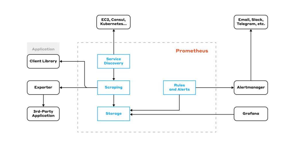
First of all, there is service discovery. It is in charge of interfacing with external API systems, such as EC2, Consul, K8s, etc. It polls these systems and compiles a list of hosts which metrics can be fetched from.
Scraping comes next. This process grabs the host list from Service Discovery and collects metrics. In Prometheus, metrics are scraped over HTTP via the pull model. In other words, Prometheus connects to endpoints and asks for metrics: “Yo, gimme the metrics!”. The app responds: “Here you go!” — and returns a page with plain text describing the metrics and their current values.
Where can Prometheus collect metrics from?
It gets them a whole group of exporters. An exporter is an application that knows how to pull metrics from different sources, such as databases or an operating system, and output them in a format that Prometheus can read.
There are tons of libraries for all kinds of frameworks that allow you to pull business metrics out of applications quickly and easily.
Once collected, the metrics need to be saved in some storage. To that end, Prometheus features its own time series database (TSDB).
Now that the metrics have been saved, they need to be analyzed. Prometheus comes with a UI that allows you to do just that. However, it is quite feature-limited: you can’t save graphs, and it comes with just one form of visualization (graph), etc. So it’s not particularly popular. Everyone uses Grafana instead.
To improve your anazyling and visualization experience, Prometheus has a built-in query language, PromQL, allowing you to extract and aggregate data. It supports both basic operations (adding or subtracting several metrics) and complex ones — calculating percentiles and quantiles, plotting sine/cosine waves, and any other functions you can think of.
On top of that, Prometheus provides rules. They allow you to define a query and store the result of that query as a new metric.
Basically, there’s a cron in there that makes a request every N seconds or minutes and saves the result as a new metric. This comes well in handy when you’re dealing with large data-loaded dashboards with complex calculations: you can retrieve the calculated metrics by running queries. That way, you get a faster display and minimize your resource usage.
PromQL also allows you to define alerts (triggers). You can specify a PromQL expression and set a threshold. When the threshold is reached, it activates the trigger and generates a notification. Prometheus does not send notifications to messengers or email — it simply generates a push request to an external system (usually Alertmanager).
Alertmanager pre-processes alerts, allowing you to build rather complex pipelines, group alerts, mute unnecessary ones, route them, and so on. The alerts can then be pushed to notify the intended recipients via messaging platforms (Slack, Mattermost, Telegram…), email, etc.
How TSDB works
In my opinion, the database is the most critical element of any monitoring system. If it’s slow, inefficient, and unreliable, the rest of the system will be slow as well. Let’s see how the database works in Prometheus and whether it fits in with our objectives.
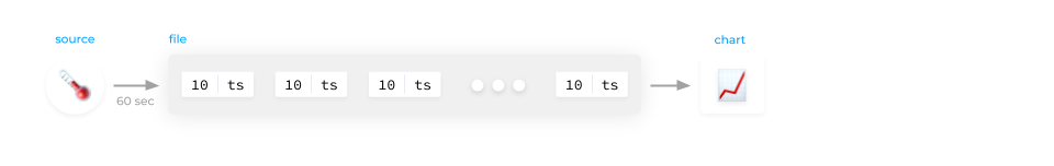
A thermometer example
Let’s start with an abstract example: suppose there is a thermometer.
- Data from its sensors are collected every 60 seconds.
- The data includes the current temperature value and the timestamp (the moment when the data was gathered).
- Both parameters are stored in a particular format (float64) and amount to 16 bytes (8 bytes for each parameter) total. Those 16 bytes are written to a file.
- A minute passes, and the next batch of data comes in and is then written to the file.
After a while, a whole hour’s worth of data is collected. Now it needs to be plotted on a graph for further study. To do so, we have to read the file (or part of it) with the necessary data and plot it on the graph with an X-axis (timestamps) and a Y-axis (temperature values).
The entire process seems to be pretty straightforward. But what if we have, say, a million data sources? What do we do in a case like that?
Let’s try to tackle the issue head-on, as we have confirmed above that writing data to a file works well. So let’s write data from each source to its own dedicated file. We’ll end up with a million different files, which is easily doable.
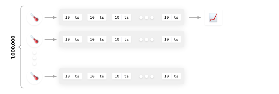
We can also easily view data from any source: open the necessary file, read the data, and plot it on a graph. Easy as pie! It all seems like a perfectly viable approach — in earlier versions, Prometheus worked roughly like this.
Actual data amount and storage challenges it brings
However, the devil is in the details — you’ve got to have them, right?
There are a million different sources, and we must write a million values into a million files once a minute. This results in a million input operations per minute, i.e., about 16,500 IOPS.
This number doesn’t seem huge — any modern SSD drive can handle it. But let’s dig a little deeper…
As previously stated, each source generates 16 bytes of data per minute (2 × float64). At 16,500 IOPS, this amounts to 22 GB per day. That number doesn’t seem excessive, either. Unfortunately, it’s not that simple.
Modern SSDs write data in blocks. Typically, these blocks are 16 KB blocks (they can be 32 KB, but that’s no matter for now). In order to write 16 bytes to the SSD, we need to read 16 KB, change 16 bytes in them and then write back those 16 KB.
Considering that, the amount of data jumps from 22 GB to 22 TB!
If you write 22 TB to an SSD daily, the drive will die soon as all SSDs have a limited number of write cycles.
And that’s just for a million sources. But what if there are 10 million sources? Then you’d have to write to SSDs at 220 TB per day… The SSD will die even sooner.
You might be thinking that a million metrics is a lot. Let’s take the following example: An empty Kubernetes cluster generates around 200,000–300,000 metrics. Meanwhile, if you add applications to it and start scaling… in a large cluster, the number of metrics can be as high as 10–15 million. What makes matters even worse is they are collected much more often than once a minute!
All of this renders our one-file-per-metric approach totally useless. However, there is another option — to write all the data to the same file.
The single-file approach
In this case, the data is written in blocks to a single file. This eliminates performance issues and prevents SSDs from dying too soon. We add data to the file periodically and end up with a set of data in a single file.
It turns out that a million records per minute will yield about 15 MB of data total and a mere 23 GB of data per day.
The question now is how to visualize the data from this file on the graph.
You have to scan the entire file, find the necessary data points in it, and plot them on the graph.
This method is more or less good for 23 GB files, but if there are 10 million sources, the file size will exceed 230 GB. The difficulty will increase even more if you need to view data for a month instead of just a day.
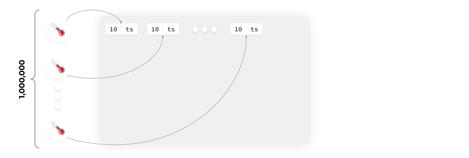
Such an approach faces obvious scalability and performance issues. That’s the problem because data is read horizontally (we need a series of data from a particular source) while it is written vertically (we collect snapshots from a large number of data sources and write them all at once).
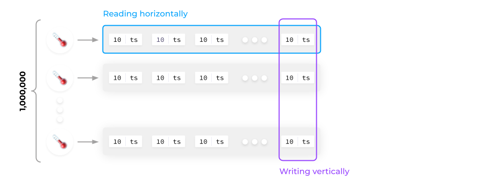
So how do you solve this conundrum? So far, we know that it is possible to write data from all sources into a single file. You can also write them to RAM grouped by time series!
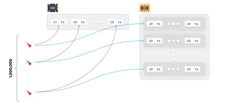
Writing metrics data to RAM
RAM is designed to handle significantly more write cycles, and because it is Random-access memory, writing to random locations is much faster in that respect. That said, it’s not good for long-term data storage — RAM is unreliable, it is likely to be cleared after a reboot, and so on. That is, while the data still needs to end up in long-term memory, you can load it from long-term storage into RAM as needed.
So the algorithm is as follows: write the collected data to the RAM, structure it there, compile a block (for example, a one-hour block), and save it to the SSD.
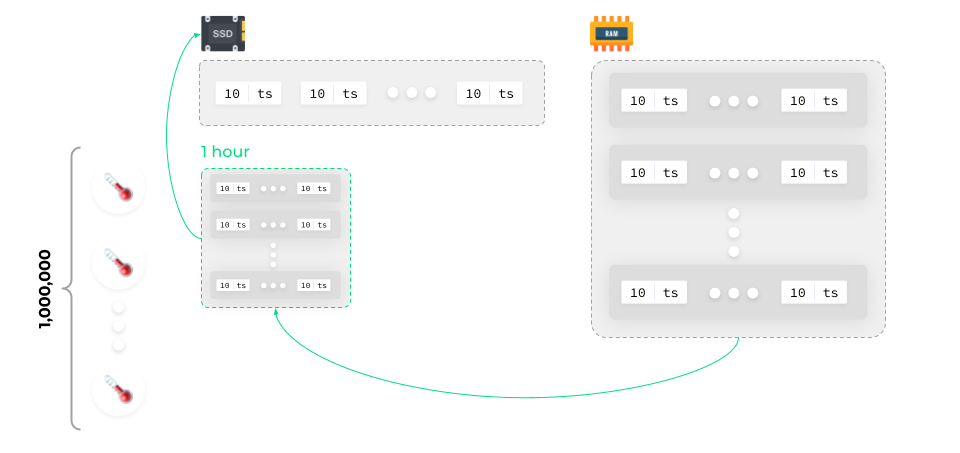
After that, the data can be cleared from the RAM. Repeat this cycle over and over again.
After a while, you’ll get a lot of information blocks saved on the SSD.
With this approach, a single 30-day month yields 720 files (1-hour file × 24 hours × 30 days). Say we want to view CPU metrics for a node. There are five metrics for the CPU: System, User, IOWait, etc. Fetching so many metrics from different blocks can overload the system.
Thus, you could, for instance, merge one-hour blocks into 4-hour blocks, then into 16-hour blocks, and so on.
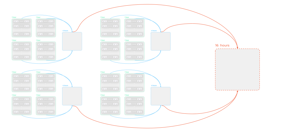
The depth of such a merge depends greatly on the TSDB implementation. They come in different flavors: some compile single-level blocks in the memory and then write them to the SSD, while others have an even deeper level of aggregation.
Such an approach completely eliminates the problem of horizontal reads and vertical writes.
However, there is another major challenge that I’ve intentionally omitted. How do you know which data belongs to which sensor? The answer is simple: label sets.
Using label sets to identify the source of data
A label set is a set of key-value pairs. Each sensor has its own label sets, allowing you to identify only a particular sensor.
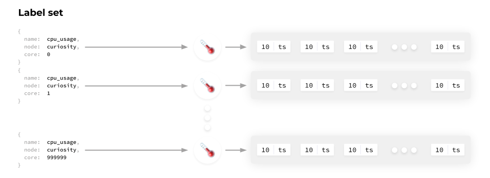
That said, storing them together with each time series is grossly inefficient and results in a significant overconsumption of resources. So, each label set gets a corresponding ID associated with it, which is then assigned to the time series.
How would it work in our case?
We have a million sensors whereby each sensor has its own label set ({ls}) and dedicated array in memory (#id). Once the data arrives, we assign an ID to each label set, then write it to the disk and save the data from that source by appending the corresponding ID to it. And then the same thing gets written into memory.
The process then repeats for all the other sources.
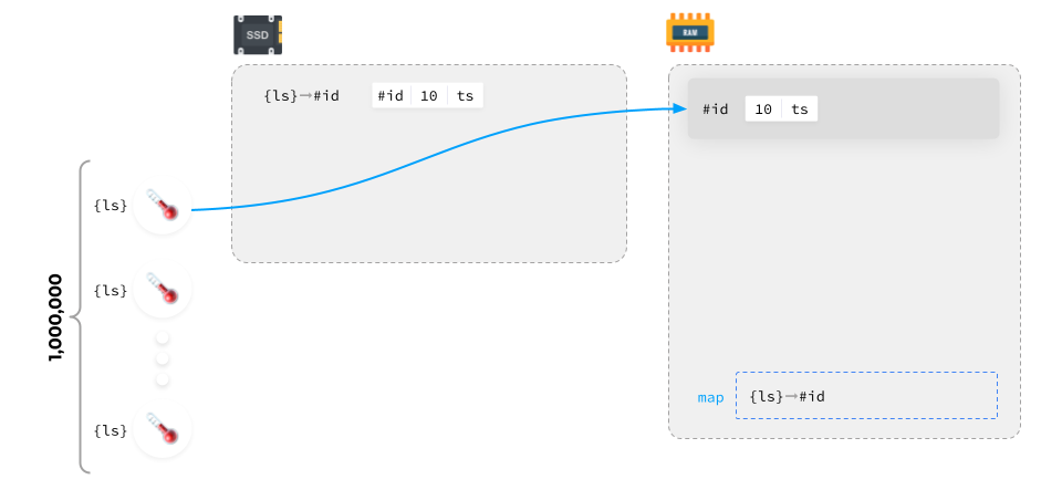
The source set generally doesn’t change much, so you don’t need to do data mapping all the time. You can just keep adding new data instead. Once the data block is compiled, it is written to the disk along with the mapping.
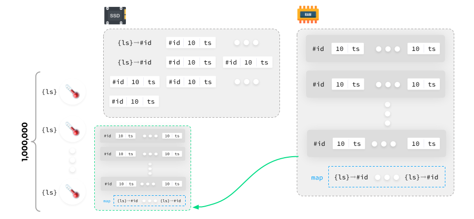
TSDB implementations do it in different ways: some use end-to-end label set numbering regardless of the block, while in other cases, label set IDs are unique to each block.
So how do you plot a graph? Suppose a request arrives to display data for a specific label set:
- The first thing to do is to figure out what the label set ID of each block is.
- Then your task is to find the matching IDs in the blocks and the fetch data.
- Finally, you can plot a graph using that data.
Done!
LSMT
So let’s summarize our experience with storing lots of metrics:
- We fixed the horizontal read and vertical write problem by “flipping” the logic to 90 degrees.
- Label sets are now used to identify the sources.
- Data is logged in series.
- The active block with data grouped by time series is kept in RAM.
- The completed blocks are written to the disk.
This approach is known as a Log-structured merge-tree (LSMT).
It is used by the majority of modern monitoring systems. For example, InfluxDB and VictoriaMetrics state this explicitly in their documentation: “We use a TSDB based on LSMT”. Prometheus doesn’t explicitly state this, but much of what is written above applies to it as well.
Conclusion
Does Prometheus meet the requirements for modern monitoring systems outlined at the beginning of this article?
Let’s check:
- Prometheus features Service discovery, which facilitates adapting to infrastructure variability.
- It provides tools for scraping metrics from applications.
- It includes a query language that allows you to aggregate metrics quickly and conveniently.
- It features a database centered around storing metrics.
- Its huge community means you can find answers to any questions you have fairly quickly.
- There is a vast number of exporters for Prometheus that allow you to monitor anything — even the water level in a bottle if that’s what you want to do.
It turns out that Prometheus meets all the requirements for a modern monitoring system and is perfectly suited to take on the lead.
In Part Two, we will learn which challenges await us with making our Prometheus metrics storage fault-tolerant and long-term and how Open Source solutions, such as Mimir, address them. UPDATE (October 26, 2023): The second part of this article, “Prometheus and centralized storage: When you need it, how it works, and what Mimir is”, is now published!

Comments